A probabilistic model for representing normally distributed subpopulations, often used for clustering.
General Principles
To discover group structures or clusters in data, we can use a Gaussian Mixture Model (GMM). This is a parametric clustering method. A GMM assumes that the data is generated from a mixture of a pre-specified number (K) of different Gaussian distributions. The model’s goal is to figure out:
The properties of each of the K clusters: For each of the K clusters, it estimates its center (mean \mu) and its shape/spread (covariance \Sigma).
The mixture weights: It estimates the proportion of the data that belongs to each cluster.
The assignment of each data point: It determines the probability of each data point belonging to each of the K clusters.
Considerations
Caution
A GMM is a Bayesian model 🛈 that considers uncertainty in all its parameters, except for the number of clusters, K, which must be fixed in advance.
The key parameters and their priors are:
Number of Clusters K: This is a fixed hyperparameter that you must choose before running the model. Choosing the right K often involves running the model multiple times and using model comparison criteria (like cross-validation, AIC, or BIC).
Cluster Weights w: These are the probabilities of drawing a data point from any given cluster. Since there are a fixed number K of them and they must sum to 1, they are typically given a Dirichlet prior. A symmetric Dirichlet prior (e.g., Dirichlet(1, 1, ..., 1)) represents an initial belief that all clusters are equally likely.
**Cluster Parameters (\mu, \Sigma): Each of the K clusters has a mean \mu and a covariance matrix \Sigma. We place priors on these to define our beliefs about their plausible values.
Like the DPMM, the model is often implemented in its marginalized form . Instead of explicitly assigning each data point to a cluster, we integrate out this choice. This creates a smoother probability surface for the inference algorithm to explore, leading to much more efficient computation.
To increase accuracy we run a k-means algorithm to initialize the cluster mean priors.
Example
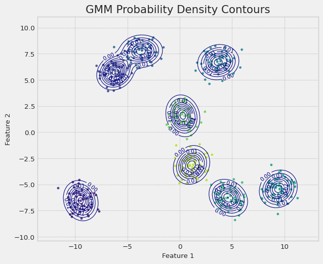
Below is an example of a GMM implemented in BI. The goal is to cluster a synthetic dataset into a pre-specified K=4 groups.
from BI import bi, jnpfrom sklearn.datasets import make_blobsm = bi()# Generate synthetic datadata, true_labels = make_blobs( n_samples=500, centers=8, cluster_std=0.8, center_box=(-10,10), random_state=101)# The modeldef gmm(data, K, initial_means): # Here K is the *exact* number of clusters D = data.shape[1] # Number of features alpha_prior =0.5* jnp.ones(K) w = m.dist.dirichlet(concentration=alpha_prior, name='weights') with m.dist.plate("components", K): # Use fixed K mu = m.dist.multivariate_normal(loc=initial_means, covariance_matrix=0.1*jnp.eye(D), name='mu') sigma = m.dist.half_cauchy(1, shape=(D,), event=1, name='sigma') Lcorr = m.dist.lkj_cholesky(dimension=D, concentration=1.0, name='Lcorr') scale_tril = sigma[..., None] * Lcorr m.dist.mixture_same_family( mixing_distribution=m.dist.categorical(probs=w, create_obj=True), component_distribution=m.dist.multivariate_normal(loc=mu, scale_tril=scale_tril, create_obj=True), name="obs", obs=data )# Kmeans clustering do initiate the meansm.ml.KMEANS(data, n_clusters=8)m.data_on_model = {"data": data,"K": 8 }m.data_on_model['initial_means'] = m.ml.results['centroids']m.fit(gmm) # Optimize model parameters through MCMC samplingm.plot(X=data,sampler=m.sampler) # Prebuild plot function for GMM
\begin{pmatrix} Y_{[i,1]} \\ \vdots \\ Y_{[i,D]} \end{pmatrix} is the i-th observation of a D-dimensional data array.
\begin{pmatrix}\mu_{[k,1]} \\ \vdots \\ \mu_{[k,D]}\end{pmatrix} is the k-th parameter vector of dimension D.
\begin{pmatrix} A_{[k,1]} \\ \vdots \\ A_{[k,D]} \end{pmatrix} is a prior for the k-th mean vector as derived by a KMEANS clustering algorithm.
B is the prior covariance of the cluster means, and is setup as a diagonal matrix with 0.1 along the diagonal.
\Sigma_k is the DxD covariance matrix of the k-th cluster (it is composed from \sigma_k and \Omega_k).
\text{Diag}(\sigma_k) is a diagonal matrix whose diagonal entries are the standard deviations:
\text{Diag}(\sigma_k) =
\begin{pmatrix}
\sigma_{[k,1]} & 0 & \cdots & 0 \\
0 & \sigma_{[k,2]} & & \vdots \\
\vdots & & \ddots & 0 \\
0 & \cdots & 0 & \sigma_{[k,D]}
\end{pmatrix}.
\sigma_{k} is a D-vector of standard deviations for the k-th cluster where each element, d, has a half-cauchy prior.
\Omega_k is a correlation matrix for the k-th cluster.
z_i is a latent variable that maps observation i to cluster k.
\pi is a vector of K cluster weights.
Where :
\begin{pmatrix} Y_{[i,1]} \\ \vdots \\ Y_{[i,D]} \end{pmatrix} is the i-th observation of a D-dimensional data array.
\begin{pmatrix}\mu_{[k,1]} \\ \vdots \\ \mu_{[k,D]}\end{pmatrix} is the k-th parameter vector of dimension D.
\begin{pmatrix} A_{[k,1]} \\ \vdots \\ A_{[k,D]} \end{pmatrix} is a prior for the k-th mean vector as derived by a KMEANS clustering algorithm.
B is the prior covariance of the cluster means, and is setup as a diagonal matrix with 0.1 along the diagonal.
\Sigma_k is the DxD covariance matrix of the k-th cluster (it is composed from \sigma_k and \Omega_k).
\sigma_k is a diagonal matrix of standard deviations for the k-th cluster.
\Omega_k is a correlation matrix for the k-th cluster.
z_i is a latent variable that maps observation i to cluster k.
\pi is a vector of K cluster weights.
Notes
Note
The primary challenge of the GMM compared to the DPMM is the need to manually specify the number of clusters K. If the chosen K is too small, the model may merge distinct clusters. If K is too large, it may split natural clusters into meaningless sub-groups. Therefore, applying a GMM often involves an outer loop of model selection where one fits the model for a range of K values and uses a scoring metric to select the best one.
Reference(s)
C. M. Bishop (2006). Pattern Recognition and Machine Learning. Springer. (Chapter 9)