Neural networks that incorporate Bayesian inference to predict probabilities across three or more mutually exclusive classes.
General Principles
Building upon the Binary Classification BNN, the BNN Multiclass Classification model can handle dependent variables with K > 2 discrete categories.
Instead of the final layer returning a single output, the final layer in a multiclass BNN returns a K-dimensional vector of scores (logits) for each observation. To transform these continuous scores into valid probabilities that sum to 1 across all K classes, we apply the softmax activation function. Finally, the categorized predictions are evaluated using a Categorical likelihood.
Considerations
Note
Output Layer Dimensions: While binary classification network predictions can be compressed to a single output logit per observation, multiclass networks MUST output exactly K dimensions in their final layer, matching the number of target classes.
The Softmax Simplex: Applying the softmax function across the final layer’s logits guarantees that the resulting outputs form a probability simplex 🛈. This is biologically similar to independent Poisson rates strictly normalizing to fixed categorical ratios.
Likelihood Function: After calculating the probabilities with softmax, we use a Categorical distribution as the final likelihood, matching the integer index of the observed category.
Improved Calibration: Multiclass BNNs greatly reduce out-of-distribution overconfidence. Standard deep learning cross-entropy models will often assign >99% probability to an unseen class purely due to the exponential nature of softmax. In a BNN, exploring the posterior width of the parameters yields “flat” unconfident probability profiles over K classes when the input is outside the training distribution.
Example
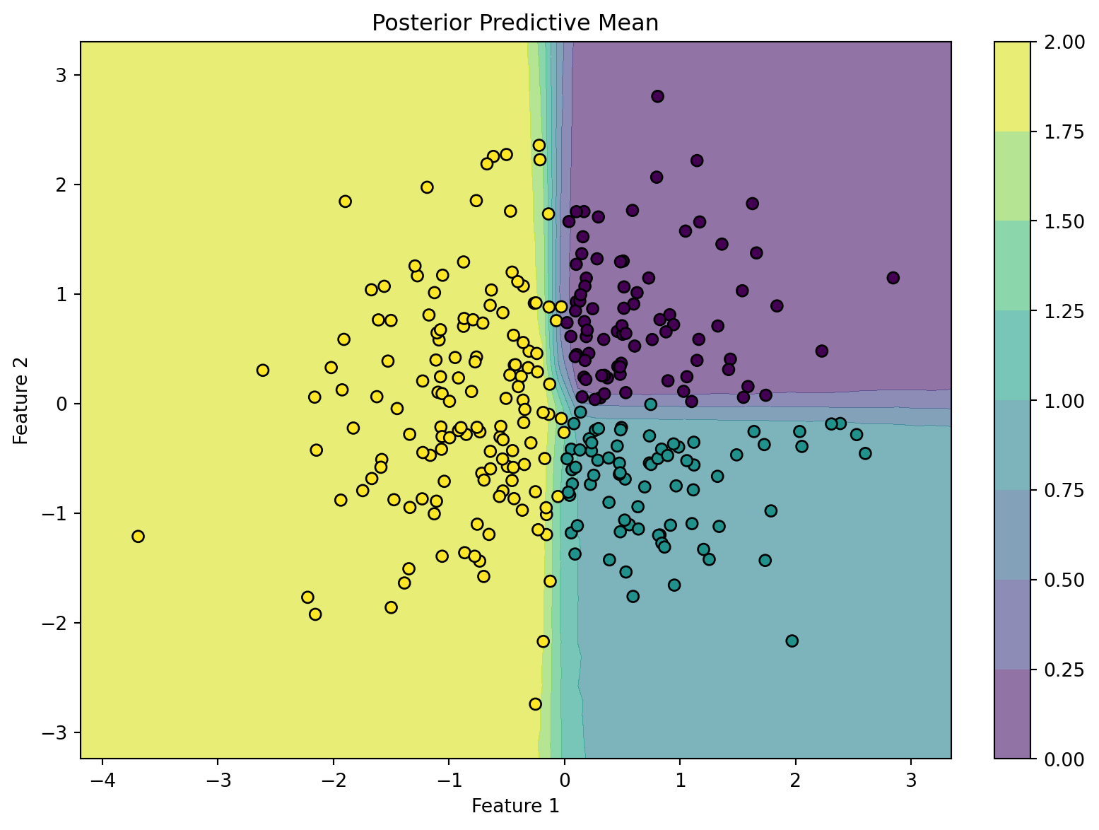
Below is an example code snippet demonstrating a Bayesian Neural Network for multiclass classification using the Bayesian Inference (BI) package. This example generates a synthetic K=3 cluster dataset.
from BI import biimport jax.numpy as jnpimport jax# Setup device------------------------------------------------m = bi(platform='cpu')# Generate Synthetic Data ------------------------------------# 3 classes based on a random normal distribution splitkey = jax.random.PRNGKey(42)X = jax.random.normal(key, (300, 2))# Rule: Q1=Class 0, Q2/Q3=Class 1, Q4=Class 2Y = jnp.where(X[:, 0] >0, jnp.where(X[:, 1] >0, 0, 1), 2)m.data_on_model =dict(X=X, Y=Y)# Define model ------------------------------------------------def model(X, Y, D_H1=5, K=3): N, D_X = X.shape# First hidden layer: 2 input features -> 5 hidden units w1 = m.bnn.layer_linear( X, dist=m.dist.normal(0, 1, name='w1_weight', shape=(D_X, D_H1)), activation='tanh' )# Final output layer: 5 hidden units -> K output units# Note: No activation is applied automatically inside the layer function here w2 = m.bnn.layer_linear( w1, dist=m.dist.normal(0, 1, name='w2_weight', shape=(D_H1, K)) )# Apply Softmax across the K dimension (axis=-1) to yield probabilities p = jax.nn.softmax(w2, axis=-1)# Categorical Likelihood matching indices in Y m.dist.categorical(probs=p, obs=Y)# Run mcmc ------------------------------------------------m.fit(model) # Approximate posterior distributions# Predictions from the model ------------------------------------------------import matplotlib.pyplot as plt# Create a grid to evaluate the modeln_grid =50x0 = jnp.linspace(X[:, 0].min() -0.5, X[:, 0].max() +0.5, n_grid)x1 = jnp.linspace(X[:, 1].min() -0.5, X[:, 1].max() +0.5, n_grid)xx0, xx1 = jnp.meshgrid(x0, x1)X_grid = jnp.c_[xx0.ravel(), xx1.ravel()]# Swap data on model temporarily to predict on the gridm.data_on_model =dict(X=X_grid, Y=jnp.zeros(X_grid.shape[0], dtype=jnp.int32))pred = m.sample(data = m.data_on_model)['x']p_mean = jnp.mean(pred, axis=0)# Plotting the posterior predictive mean (categorical blending)fig, ax = plt.subplots(figsize=(8, 6), constrained_layout=True)contour = ax.contourf(xx0, xx1, p_mean.reshape(n_grid, n_grid), cmap="viridis", alpha=0.6)scatter = ax.scatter(X[:, 0], X[:, 1], c=Y, cmap="viridis", edgecolors='k')ax.set(title="Posterior Predictive Mean", xlabel="Feature 1", ylabel="Feature 2")fig.colorbar(contour, ax=ax)
/home/sosa/work/3.12venv/lib/python3.10/site-packages/tqdm/auto.py:21: TqdmWarning:

IProgress not found. Please update jupyter and ipywidgets. See https://ipywidgets.readthedocs.io/en/stable/user_install.html
BI v 0.0.45 package loaded
jax.local_device_count 32
⚠️This function is still in development. Use it with caution. ⚠️
⚠️This function is still in development. Use it with caution. ⚠️
⚠️This function is still in development. Use it with caution. ⚠️
⚠️This function is still in development. Use it with caution. ⚠️
⚠️This function is still in development. Use it with caution. ⚠️
⚠️This function is still in development. Use it with caution. ⚠️
usingBayesianInferenceusingPythonCall# Setup device------------------------------------------------m =importBI(platform="cpu")# Generate Synthetic Data ------------------------------------np =pyimport("numpy")jax_random =pyimport("jax.random")jnp =pyimport("jax.numpy")key = jax_random.PRNGKey(42)X = jax_random.normal(key, (300, 2))# Simple rule to partition into K=3 classesY = jnp.where(X[:, 0] >0, jnp.where(X[:, 1] >0, 0, 1), 2)m.data_on_model["X"] = Xm.data_on_model["Y"] = Y# Define model ------------------------------------------------@BIfunctionmodel(X, Y) N, D_X =size(X) D_H1 =5 K =3# First hidden layer w1 = m.bnn.layer_linear( X, dist=m.dist.normal(0, 1, name="w1_weight", shape=(D_X, D_H1)), activation="tanh" )# Final output layer w2 = m.bnn.layer_linear( w1, dist=m.dist.normal(0, 1, name="w2_weight", shape=(D_H1, K)) )# Softmax conversion to probability simplex p = jax.nn.softmax(w2, axis=-1)# Categorical Likelihood m.dist.categorical(probs=p, obs=Y)end# Run mcmc ------------------------------------------------m.fit(model, num_samples=500, progress_bar=false)
Mathematical Details
Bayesian Formulation
For a multiclass classification task spanning N observations and K mutually exclusive classes, we model the probability vector \theta_i that the response Y_i \in \{0, 1, ..., K-1\} falls into each respective class.
Using a single hidden layer with a hyperbolic tangent (\tanh) activation function, the model is structured as:
Y_i is the observed class index for the i-th observation (Y_i \in \{0, 1, ..., K-1\}).
\theta_i is the predicted probability vector for the i-th observation.
\phi_i are the K-dimensional logits.
X_i is the input row vector for the i-th observation, with features length D_X = 2.
H_i is the hidden layer representation vector for the i-th observation. It has length D_H = 5.
\Theta_1 is the weight matrix of the first hidden layer (2 \times 5).
\Theta_2 is the final layer weight matrix mapping the hidden features to the logits for the K=3 classes (5 \times 3).
All elements within the weight matrices \Theta_1 and \Theta_2 are assigned independent standard Normal priors.
Notes
Note
For large outputs where K > 100, computing the exact softmax normalization scalar (the denominator term combining all exponentiated logits) can become computationally expensive over thousands of MCMC posterior evaluations.
Neural networks configured with a standard Cross-Entropy loss mapping to one-hot vectors conceptually perform exactly this sequence: dot product of final weights \rightarrow Softmax \rightarrow Categorical Likelihood.