Neural networks that incorporate Bayesian inference to quantify uncertainty in their predictions.
General Principles
To model complex, non-linear relationships between variables, we can use multiple approaches including, splines, polynomials, gaussian processes, and neural networks. Here, we will focus on a Bayesian Neural Network (BNN). Think of a neural network as a highly flexible function made of interconnected layers of “neurons.” Each connection between neurons has a weight, and each neuron has a bias. These weights and biases are like a vast set of adjustable knobs. In a standard network, the goal is to find the single best setting for all these knobs to map inputs to outputs. Unlike a standard neural network which learns a single set of optimal weights, a BNN learns distributions over its weights and biases. This allows it to capture not just the relationship in the data, but also its own uncertainty about that relationship. For this, we need to define:
A Network Architecture, which specifies the number of layers, the number of neurons in each layer, and the activation functions (e.g., ReLU, tanh) that introduce non-linearity. This defines the structure of our “knobs.”
Priors for Arrays of Weights and Biases. In a simple model like linear regression, we define a prior for each individual parameter (e.g., one prior for the slope \beta). In a neural network, which can have thousands or millions of weights, we don’t define a unique prior for every single one. Instead, we define a prior that acts as a template for an entire array of parameters. For example, we might declare that all weights in a specific layer are drawn from the same Normal(0, 1) distribution. This allows us to efficiently specify our beliefs about the entire set of network parameters.
An Output Distribution (Likelihood), which defines the probability of the data given the network’s predictions. For a continuous variable (regression), this is often a Normal distribution with a variance term \sigma that quantifies the data’s noise around the model’s predictions.
Considerations
Caution
Like all Bayesian models, BNNs consider model parameter uncertainty 🛈. The parameters here are the network’s weights (W) and biases (b). We quantify our uncertainty about them through their posterior distribution 🛈. Therefore, we must declare prior distributions 🛈 for all weights and biases, as well as for the output variance \sigma.
Unlike in a linear regression where the coefficient \beta has a direct interpretation (e.g., the effect of weight on height), the individual weights and biases in a BNN are not directly interpretable. A single weight’s influence is entangled with thousands of other parameters through non-linear functions. Consequently, BNNs are best viewed as powerful predictive tools rather than explanatory ones. They excel at learning complex patterns and quantifying predictive uncertainty, but if the goal is to isolate and interpret the effect of a specific variable, a simpler model is often more appropriate.
Prior distributions are built following these considerations:
As the data is typically scaled 🛈 (see introduction), we can use a standard Normal distribution (mean 0, standard deviation 1) as a weakly-informative prior for all weights and biases. This acts as a form of regularization.
Since the output variance \sigma must be positive, we can use a positively-defined distribution, such as the Exponential or Half-Normal.
BNNs can be used for both regression and classification. The final layer’s activation and the chosen likelihood distribution depend on the task. For binary classification, a sigmoid activation is paired with a Bernoulli likelihood, which requires a link function 🛈 (logit) to connect the linear output of the network to the probability space [0, 1]. For regression, the identity activation is often used with a Gaussian likelihood.
Example
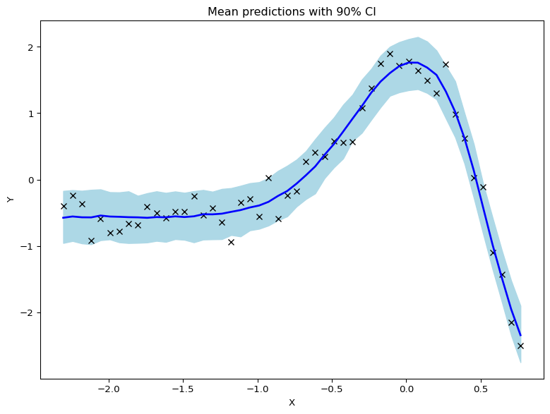
Below is an example code snippet demonstrating a Bayesian Neural Network for regression using the Bayesian Inference (BI) package. Data consist of two continuous variables (height and weight), and the goal is to predict height from weight using a non-linear model.
from BI import biimport jsonimport jax.numpy as jnpimport matplotlib.pyplot as plt# Setup device------------------------------------------------m = bi(platform='cpu')# Import Data & Data Manipulation ------------------------------------------------withopen('BNN.json', 'r', encoding='utf-8') asfile:# Load the JSON data into a Python dictionary data = json.load(file)# X is already scaledX = jnp.array(data['X']) # Note X shape = (N,2) where first column is the intercept and second column is the predictorY = jnp.array(data['Y']) # Note Y shape = (N,1) where N is the number of observationsm.data_on_model =dict(X = X, Y = Y)# Define model ------------------------------------------------def model(X, Y, D_H=5, D_Y=1): N, D_X = X.shape# First hidden layer: Transforms input to N × D_H (hidden units) w1 = m.bnn.layer_linear( X, dist=m.dist.normal(0, 1, name='w1',shape=(D_X,D_H) ), activation='tanh' )# sample final layer of weights and neural network output# Final layer (z3) computes linear combination of second hidden layer w2 = m.bnn.layer_linear( X=w1, dist=m.dist.normal(0, 1, name='w2',shape=(D_H,D_Y)) ) sigma = m.dist.exponential(1, name='sigma') m.dist.normal(w2, sigma, obs=Y,name='Y')# Run mcmc ------------------------------------------------m.fit(model, num_samples=500, progress_bar=False) # Approximate posterior distributions for weights, biases, and sigma# Predictions from the model ------------------------------------------------pred = m.sample(samples =500)['Y']pred = pred[..., 0]mean_prediction = jnp.mean(pred, axis=0)percentiles = jnp.percentile(pred, jnp.array([5.0, 95.0]), axis=0)# make plotsfig, ax = plt.subplots(figsize=(8, 6), constrained_layout=True)# plot training dataax.plot(X[:, 1], Y[:, 0], "kx")# plot 90% confidence level of predictionsax.fill_between( X[:, 1], percentiles[0, :], percentiles[1, :], color="lightblue")# plot mean predictionax.plot(X[:, 1], mean_prediction, "blue", ls="solid", lw=2.0)ax.set(xlabel="X", ylabel="Y", title="Mean predictions with 90% CI")
jax.local_device_count 16
⚠️This function is still in development. Use it with caution. ⚠️
⚠️This function is still in development. Use it with caution. ⚠️
⚠️This function is still in development. Use it with caution. ⚠️
⚠️This function is still in development. Use it with caution. ⚠️
⚠️This function is still in development. Use it with caution. ⚠️
⚠️This function is still in development. Use it with caution. ⚠️
⚠️This function is still in development. Use it with caution. ⚠️
⚠️This function is still in development. Use it with caution. ⚠️
library(BayesianInference)m=importBI(platform='cpu')# Load csv file# Import data ------------------------------------------------path =normalizePath(paste(system.file(package ="BayesianInference"),"/data/BNN.json", sep =''))data <-fromJSON(path)m$data_on_model =list()m$data_on_model$X = jnp$array(data$X)m$data_on_model$Y = jnp$array(data$Y)# Define model ------------------------------------------------model <-function(X, Y, D_X =2, D_H=5L, D_Y=1L){ w1 <- m$bnn$layer_linear(X, dist=bi.dist.normal(0, 1, name='w1',shape=c(D_X,D_H)), activation='tanh') w2 <- m$bnn$layer_linear( w1, dist=bi.dist.normal(0, 1, name='w2',shape=c(D_H,D_Y)),activation='tanh' )# Prior for the output standard deviation s =bi.dist.exponential(1, name ='s')# Likelihoodbi.dist.normal(w2, s, obs = Y)}# Run mcmc ------------------------------------------------m$fit(model) # Approximate posterior distributions
Mathematical Details
Notes
Note
The primary difference between a Frequentist and Bayesian neural network lies in how parameters are treated. In the frequentist approach, weights and biases are point estimates found by minimizing a loss function (e.g., via gradient descent). Techniques like Dropout or L2 regularization are often used to prevent overfitting, which can be interpreted as approximations to a Bayesian treatment. In contrast, the Bayesian formulation does not seek a single best set of weights. Instead, it uses methods like MCMC or Variational Inference to approximate the entire posterior distribution for every weight and bias. This provides a principled and direct way to quantify model uncertainty.
While present an example of non-linear regression, the Bayesian Neural Network can be used for linear regressions as well (keeping in mind that interpretation of the weights are impossible).